Practice Exercise 2 (45 Questions)
45 advanced CAT-level line graph questions covering multi-variable systems, index conversions, and cumulative curves.
Practice Exercise 2 — Advanced & Past CAT Sets
45 high-difficulty questions.
Practice questions
Question 1 · Moderate
Directions for Questions 1 to 6
Answer the questions on the basis of the information given below.
An industrial sustainable materials and engineered composites conglomerate, SylvaTech Biomaterials, tracks wholesale procurement spot prices across three core raw material processing categories: Plywood, Saw Timber, and Logs from 1987 to 1993.
In the line graph below, the benchmark price of roundwood logs is quoted per cubic metre (Rs./m³), while the prices of engineered plywood and milled saw timber are quoted per metric tonne (Rs./tonne).
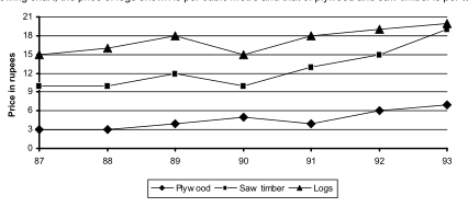
What is the maximum percentage increase in price per cubic metre or per tonne over the previous year across any of the three material categories?
Show answer and explanation
Answer: (C) 50%
To determine the maximum year-on-year percentage increase across all three product categories, we compile the yearly benchmark prices and compute their percentage growth rates:
| Year | Plywood (Rs./tonne) | Saw timber (Rs./tonne) | Logs (Rs./m³) | |||
|---|---|---|---|---|---|---|
| Price | % Increase | Price | % Increase | Price | % Increase | |
| 1987 | 3 | — | 10 | — | 15 | — |
| 1988 | 3 | 0% | 10 | 0% | 16 | 6.67% |
| 1989 | 4 | 33.33% | 12 | 20.00% | 18 | 12.50% |
| 1990 | 5 | 25.00% | 10 | — | 15 | — |
| 1991 | 4 | — | 13 | 30.00% | 18 | 20.00% |
| 1992 | 6 | 50.00% | 15 | 15.38% | 19 | 5.55% |
| 1993 | 7 | 16.67% | 19 | 26.67% | 20 | 5.26% |
From the tabulated data, the highest annual growth rate is 50%, occurring for Plywood in 1992 (rising from Rs. 4 to Rs. 6 per tonne).
Question 2 · Moderate
Directions for Questions 1 to 6
Answer the questions on the basis of the information given below.
An industrial sustainable materials and engineered composites conglomerate, SylvaTech Biomaterials, tracks wholesale procurement spot prices across three core raw material processing categories: Plywood, Saw Timber, and Logs from 1987 to 1993.
In the line graph below, the benchmark price of roundwood logs is quoted per cubic metre (Rs./m³), while the prices of engineered plywood and milled saw timber are quoted per metric tonne (Rs./tonne).
Which material product demonstrates the maximum percentage increase in price over the entire seven-year period from 1987 to 1993?
Show answer and explanation
Answer: (B) Plywood
We calculate the overall net percentage increase from 1987 to 1993 for each material category:
| Material Category | Price in 1987 | Price in 1993 | Net Calculation | Percentage Growth |
|---|---|---|---|---|
| Plywood | Rs. 3 | Rs. 7 | $$\frac{7 - 3}{3} \times 100$$ | 133.33% |
| Saw timber | Rs. 10 | Rs. 19 | $$\frac{19 - 10}{10} \times 100$$ | 90.00% |
| Logs | Rs. 15 | Rs. 20 | $$\frac{20 - 15}{15} \times 100$$ | 33.33% |
Thus, Plywood experienced the highest overall percentage appreciation across the entire seven-year period (133.33%).
Question 3 · Moderate
Directions for Questions 1 to 6
Answer the questions on the basis of the information given below.
An industrial sustainable materials and engineered composites conglomerate, SylvaTech Biomaterials, tracks wholesale procurement spot prices across three core raw material processing categories: Plywood, Saw Timber, and Logs from 1987 to 1993.
In the line graph below, the benchmark price of roundwood logs is quoted per cubic metre (Rs./m³), while the prices of engineered plywood and milled saw timber are quoted per metric tonne (Rs./tonne).
If for saw timber, in which year was the absolute difference between the per cubic metre prices of saw timber and logs the least?
Show answer and explanation
Answer: (B) 1990
Since saw timber is quoted in Rs./tonne and logs in Rs./m³, we standardize saw timber into Rs./m³:
Given: .
Now we evaluate the absolute difference between saw timber and logs per cubic metre across the four options:
| Year | Saw Timber (Rs./tonne) | Saw Timber (Rs./m³) | Logs (Rs./m³) | Absolute Difference |
|---|---|---|---|---|
| 1989 | 12 | $12 \times 0.75 = 9.00$ | 18 | $|9.00 - 18| = 9.00$ |
| 1990 | 10 | $10 \times 0.75 = 7.50$ | 15 | $|7.50 - 15| = \mathbf{7.50}$ |
| 1991 | 13 | $13 \times 0.75 = 9.75$ | 18 | $|9.75 - 18| = 8.25$ |
| 1992 | 15 | $15 \times 0.75 = 11.25$ | 19 | $|11.25 - 19| = 7.75$ |
The price difference was smallest in 1990 at Rs. 7.50 per cubic metre.
Question 4 · Moderate
Directions for Questions 1 to 6
Answer the questions on the basis of the information given below.
An industrial sustainable materials and engineered composites conglomerate, SylvaTech Biomaterials, tracks wholesale procurement spot prices across three core raw material processing categories: Plywood, Saw Timber, and Logs from 1987 to 1993.
In the line graph below, the benchmark price of roundwood logs is quoted per cubic metre (Rs./m³), while the prices of engineered plywood and milled saw timber are quoted per metric tonne (Rs./tonne).
If one cubic metre equals for plywood and for saw timber, in which year was the difference in the prices of plywood and saw timber (per cubic metre) the maximum?
Show answer and explanation
Answer: (D) 1992
Using the volumetric density conversions:
-
Plywood:
-
Saw timber:
We calculate the volumetric prices and absolute difference for each candidate year:
| Year | Saw Timber (Rs./tonne) | Saw Timber (Rs./m³) | Plywood (Rs./tonne) | Plywood (Rs./m³) | Difference (Rs./m³) |
|---|---|---|---|---|---|
| 1989 | 12 | $12 \times 0.8 = 9.60$ | 4 | $4 \times 0.7 = 2.80$ | $9.60 - 2.80 = 6.80$ |
| 1990 | 10 | $10 \times 0.8 = 8.00$ | 5 | $5 \times 0.7 = 3.50$ | $8.00 - 3.50 = 4.50$ |
| 1991 | 13 | $13 \times 0.8 = 10.40$ | 4 | $4 \times 0.7 = 2.80$ | $10.40 - 2.80 = 7.60$ |
| 1992 | 15 | $15 \times 0.8 = 12.00$ | 6 | $6 \times 0.7 = 4.20$ | $12.00 - 4.20 = \mathbf{7.80}$ |
The difference between the two prices per cubic metre reached its maximum in 1992 at Rs. 7.80.
Question 5 · Moderate
Directions for Questions 1 to 6
Answer the questions on the basis of the information given below.
An industrial sustainable materials and engineered composites conglomerate, SylvaTech Biomaterials, tracks wholesale procurement spot prices across three core raw material processing categories: Plywood, Saw Timber, and Logs from 1987 to 1993.
In the line graph below, the benchmark price of roundwood logs is quoted per cubic metre (Rs./m³), while the prices of engineered plywood and milled saw timber are quoted per metric tonne (Rs./tonne).
If the total volume procurement sales of plywood, saw timber, and logs were distributed in the ratio of , , and respectively, what was the weighted average sales realization in 1993 per cubic metre of sales? (Assume the density of one cubic metre of both saw timber and plywood is )
Show answer and explanation
Answer: (D) 13
Given that (or , so density factor ):
From the 1993 graph values:
-
Logs: Rs. 20 per m³
-
Plywood: Rs. 7 per tonne
-
Saw timber: Rs. 19 per tonne
With sales volume weights in the ratio ():
Hence, the average realization is approximately 13.
Question 6 · Moderate
Directions for Questions 1 to 6
Answer the questions on the basis of the information given below.
An industrial sustainable materials and engineered composites conglomerate, SylvaTech Biomaterials, tracks wholesale procurement spot prices across three core raw material processing categories: Plywood, Saw Timber, and Logs from 1987 to 1993.
In the line graph below, the benchmark price of roundwood logs is quoted per cubic metre (Rs./m³), while the prices of engineered plywood and milled saw timber are quoted per metric tonne (Rs./tonne).
Referring to the procurement distribution in the previous question, if in 1994 the per cubic metre prices of plywood, saw timber, and logs increased by , , and respectively while the volume sales proportion remained at , , and , what was the revised average realization per cubic metre?
Show answer and explanation
Answer: (C) 13.15
Adjusting the 1993 per-m³ price components by their respective percentage increases for 1994:
-
Plywood:
-
Saw timber:
-
Logs:
Calculating the revised weighted average realization with weights :
Hence, the revised realization is 13.15.
Question 7 · Moderate
Directions for Questions 7 to 10
Answer the questions on the basis of the information given below.
In autonomous robotics and digital signal processing, calibration algorithms evaluate continuous sensor input response waveforms against transformed filtering transfer functions . Both waveforms are defined across the standardized operational domain and consist of continuous piecewise linear segments.
For each question, inspect the given pair of response profiles and select:
-
(1) if
-
(2) if
-
(3) if
-
(4) if none of the above is true
Inspect the sensor calibration waveforms and shown below:
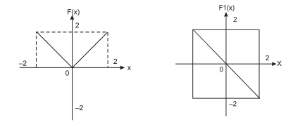
Which functional transformation describes the relationship between and ?
Show answer and explanation
Answer: (D) if none of the above is true
Analyzing the piecewise graphs:
-
represents the absolute value profile , with , , and .
-
represents the linear ramp , with , , and .
We test each proposed mathematical relation:
-
If :
At , , whereas . (False)
-
If :
At , , whereas . (False)
-
If :
At , , whereas . (False)
Since none of the three relationships is universally satisfied across , the correct option is (4) if none of the above is true.
Question 8 · Moderate
Directions for Questions 7 to 10
Answer the questions on the basis of the information given below.
In autonomous robotics and digital signal processing, calibration algorithms evaluate continuous sensor input response waveforms against transformed filtering transfer functions . Both waveforms are defined across the standardized operational domain and consist of continuous piecewise linear segments.
For each question, inspect the given pair of response profiles and select:
-
(1) if
-
(2) if
-
(3) if
-
(4) if none of the above is true
Inspect the sensor calibration waveforms and shown below:
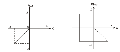
Which functional transformation describes the relationship between and ?
Show answer and explanation
Answer: (B) if F1(x) = F(–x)
From the piecewise graphs:
-
is defined as:
-
is defined as:
Evaluating :
-
When , .
-
When , .
Testing coordinates:
-
At : ; .
-
At : ; .
Because holds across all , the correct option is (2) if F1(x) = F(–x).
Question 9 · Moderate
Directions for Questions 7 to 10
Answer the questions on the basis of the information given below.
In autonomous robotics and digital signal processing, calibration algorithms evaluate continuous sensor input response waveforms against transformed filtering transfer functions . Both waveforms are defined across the standardized operational domain and consist of continuous piecewise linear segments.
For each question, inspect the given pair of response profiles and select:
-
(1) if
-
(2) if
-
(3) if
-
(4) if none of the above is true
Inspect the sensor calibration waveforms and shown below:
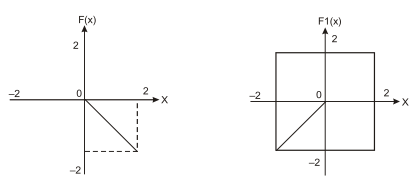
Which functional transformation describes the relationship between and ?
Show answer and explanation
Answer: (B) if F1(x) = F(–x)
From the piecewise graphs:
-
is defined as:
-
is defined as:
Replacing with in :
-
For , .
-
For , .
Testing coordinates:
-
At : ; .
-
At : ; .
Thus holds across the entire domain. Hence, the correct choice is (2) if F1(x) = F(–x).
Question 10 · Moderate
Directions for Questions 7 to 10
Answer the questions on the basis of the information given below.
In autonomous robotics and digital signal processing, calibration algorithms evaluate continuous sensor input response waveforms against transformed filtering transfer functions . Both waveforms are defined across the standardized operational domain and consist of continuous piecewise linear segments.
For each question, inspect the given pair of response profiles and select:
-
(1) if
-
(2) if
-
(3) if
-
(4) if none of the above is true
Inspect the sensor calibration waveforms and shown below:
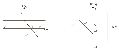
Which functional transformation describes the relationship between and ?
Show answer and explanation
Answer: (C) if F1(x) = –F(–x)
Evaluating the characteristic coordinates from both graphs:
-
For :
- , ,
-
For :
- , ,
Let us test the relation :
-
At : and . (Satisfied)
-
At : and . (Satisfied)
-
At : and . (Satisfied)
Because matches all coordinates and piecewise linear slopes, the correct option is (3) if F1(x) = –F(–x).
Question 11 · Moderate
Directions for Questions 11 and 12
Answer the questions on the basis of the information given below.
Two autonomous electric-hybrid transit vehicles operated by field test engineers Rohan and Aditi are evaluated on a standardized highway proving corridor between Terminal Alpha and Terminal Beta.
-
Rohan completes the journey from Terminal Alpha to Terminal Beta in exactly 4 hours, maintaining a constant cruising speed of for the first two hours and for the remaining two hours.
-
Aditi travels along the exact same corridor but drives across three distinct velocity segments: , , and , covering an identical distance in each speed segment.
Both vehicles share identical powertrain efficiency characteristics, where fuel economy (kilometres per litre) varies non-linearly with cruising speed as depicted in the graph below.
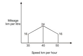
What is the total quantity of fuel consumed by Aditi's vehicle for the entire journey from Terminal Alpha to Terminal Beta?
Show answer and explanation
Answer: (C) 8.9 l
-
Determine Total Distance:
From Rohan's trip:
-
Aditi's Segment Distances:
Aditi divides the 160 km trip into three equal distance segments:
-
Fuel Consumption per Segment:
From the powertrain mileage curve:
-
At : Mileage
-
At : Mileage
-
At : Mileage
-
-
Total Fuel Consumed:
Hence, Aditi consumed 8.9 l of fuel.
Question 12 · Moderate
Directions for Questions 11 and 12
Answer the questions on the basis of the information given below.
Two autonomous electric-hybrid transit vehicles operated by field test engineers Rohan and Aditi are evaluated on a standardized highway proving corridor between Terminal Alpha and Terminal Beta.
-
Rohan completes the journey from Terminal Alpha to Terminal Beta in exactly 4 hours, maintaining a constant cruising speed of for the first two hours and for the remaining two hours.
-
Aditi travels along the exact same corridor but drives across three distinct velocity segments: , , and , covering an identical distance in each speed segment.
Both vehicles share identical powertrain efficiency characteristics, where fuel economy (kilometres per litre) varies non-linearly with cruising speed as depicted in the graph below.
Telemetry engineer Zoheb plans to drive Aditi’s vehicle over the exact same route from Terminal Alpha to Terminal Beta while strictly minimizing total fuel consumption. What is the minimum quantity of fuel required by Zoheb?
Show answer and explanation
Answer: (A) 6.67 l
To minimize total fuel consumption over the 160 km distance, Zoheb must operate the vehicle at the cruising speed that maximizes fuel efficiency (highest km per litre).
From the graph:
- Maximum fuel efficiency is 24 km per litre, achieved at a steady speed of 40 km/h.
Hence, Zoheb requires 6.67 l of fuel.
Question 13 · Moderate
Directions for Questions 13 to 16
Answer the questions on the basis of the information given below.
The line graph below illustrates the annual revenue (sales) and net profit (in Rs. crore) of enterprise cloud infrastructure provider IVP Cloud Systems across five consecutive fiscal years from 1994-95 to 1998-99.
During this five-year operational horizon, annual sales surged from Rs. 100 crore to Rs. 680 crore, while annual net profit expanded from Rs. 2.5 crore to Rs. 12 crore.
Net profit is defined as the surplus of sales revenue over total operating costs:
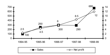
The highest annual percentage growth rate in sales revenue, relative to the immediately preceding fiscal year, occurred in:
Show answer and explanation
Answer: (A) 1995-96
From the sales revenue line graph, we compute year-on-year growth across all fiscal periods:
| Fiscal Year | Previous Sales (Rs. cr) | Current Sales (Rs. cr) | Absolute Increase | Percentage Growth |
|---|---|---|---|---|
| 1995-96 | 100 | 250 | +150 | $$\frac{150}{100} \times 100 = \mathbf{150.0\%}$$ |
| 1996-97 | 250 | 300 | +50 | $$\frac{50}{250} \times 100 = 20.0\%$$ |
| 1997-98 | 300 | 290 | -10 | $$-3.33\%$$ |
| 1998-99 | 290 | 680 | +390 | $$\frac{390}{290} \times 100 \approx 134.48\%$$ |
The highest percentage growth relative to the previous year occurred in 1995-96 (150%).
Question 14 · Moderate
Directions for Questions 13 to 16
Answer the questions on the basis of the information given below.
The line graph below illustrates the annual revenue (sales) and net profit (in Rs. crore) of enterprise cloud infrastructure provider IVP Cloud Systems across five consecutive fiscal years from 1994-95 to 1998-99.
During this five-year operational horizon, annual sales surged from Rs. 100 crore to Rs. 680 crore, while annual net profit expanded from Rs. 2.5 crore to Rs. 12 crore.
Net profit is defined as the surplus of sales revenue over total operating costs:
The highest annual percentage growth rate in net profit, relative to the immediately preceding fiscal year, was achieved in:
Show answer and explanation
Answer: (D) 1995-96
From the net profit line graph, the net profit values (in Rs. crore) are:
-
1994-95: Rs. 2.5 cr
-
1995-96: Rs. 4.5 cr
-
1996-97: Rs. 6.0 cr
-
1997-98: Rs. 8.5 cr
-
1998-99: Rs. 12.0 cr
Computing annual growth in net profit:
| Fiscal Year | Previous Profit | Current Profit | Absolute Increase | Percentage Growth |
|---|---|---|---|---|
| 1995-96 | 2.5 | 4.5 | +2.0 | $$\frac{2.0}{2.5} \times 100 = \mathbf{80.0\%}$$ |
| 1996-97 | 4.5 | 6.0 | +1.5 | $$\frac{1.5}{4.5} \times 100 = 33.33\%$$ |
| 1997-98 | 6.0 | 8.5 | +2.5 | $$\frac{2.5}{6.0} \times 100 = 41.67\%$$ |
| 1998-99 | 8.5 | 12.0 | +3.5 | $$\frac{3.5}{8.5} \times 100 = 41.18\%$$ |
The highest percentage expansion in net profit was achieved in 1995-96 (80%).
Question 15 · Moderate
Directions for Questions 13 to 16
Answer the questions on the basis of the information given below.
The line graph below illustrates the annual revenue (sales) and net profit (in Rs. crore) of enterprise cloud infrastructure provider IVP Cloud Systems across five consecutive fiscal years from 1994-95 to 1998-99.
During this five-year operational horizon, annual sales surged from Rs. 100 crore to Rs. 680 crore, while annual net profit expanded from Rs. 2.5 crore to Rs. 12 crore.
Net profit is defined as the surplus of sales revenue over total operating costs:
Defining operating profitability as the ratio of net profit to annual sales, IVP Cloud Systems recorded its highest profitability margin in:
Show answer and explanation
Answer: (B) 1997-98
Profitability ratio is defined as .
Evaluating the profitability metric across all five years:
| Fiscal Year | Net Profit (Rs. cr) | Sales (Rs. cr) | Profitability Ratio | Profitability Margin (%) |
|---|---|---|---|---|
| 1994-95 | 2.5 | 100 | 0.0250 | 2.50% |
| 1995-96 | 4.5 | 250 | 0.0180 | 1.80% |
| 1996-97 | 6.0 | 300 | 0.0200 | 2.00% |
| 1997-98 | 8.5 | 290 | 0.0293 | 2.93% |
| 1998-99 | 12.0 | 680 | 0.0176 | 1.76% |
The company recorded its peak profitability margin in 1997-98 (approximately 2.93%).
Question 16 · CAT Level
Directions for Questions 13 to 16
Answer the questions on the basis of the information given below.
The line graph below illustrates the annual revenue (sales) and net profit (in Rs. crore) of enterprise cloud infrastructure provider IVP Cloud Systems across five consecutive fiscal years from 1994-95 to 1998-99.
During this five-year operational horizon, annual sales surged from Rs. 100 crore to Rs. 680 crore, while annual net profit expanded from Rs. 2.5 crore to Rs. 12 crore.
Net profit is defined as the surplus of sales revenue over total operating costs:
With profitability defined as the ratio of net profit to annual sales as in the previous question, which of the following statements can be correctly inferred regarding the trend over the five-year period?
Show answer and explanation
Answer: (D) None of the above
From our calculation of the profitability series across the five years:
-
1994-95:
-
1995-96: (decrease)
-
1996-97: (increase)
-
1997-98: (increase)
-
1998-99: (decrease)
Because profitability alternately decreases, increases, and decreases again, it is neither monotonically non-decreasing, nor monotonically non-increasing, nor constant.
Hence, the correct conclusion is (4) None of the above.
Question 17 · CAT Level
Directions for Questions 17 to 20
Answer the questions on the basis of the information given below.
Quantitative multi-asset fund Aegis Capital monitors high-frequency price fluctuations across four core commodity asset classes — Arhar, Pepper, Sugar, and Gold — over bi-weekly valuation cycles from February to July 1999 as presented in the graphs below.
Benchmark spot pricing is quoted in:
-
Rs. per quintal for Arhar and Sugar
-
Rs. per kg for Pepper
-
Rs. per 10 grams for Gold
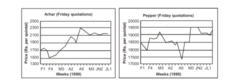
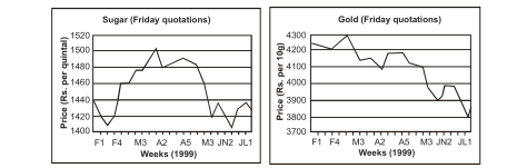
The price change of a commodity is defined as the absolute difference between ending and beginning prices, expressed as a percentage of the beginning price. Which commodity registered the highest price change over the February–July period?
Show answer and explanation
Answer: (A) Arhar
Reading the beginning (early February, F1) and ending (early July, JL1) prices from the charts for each commodity:
| Commodity | Beginning Price | Ending Price | Absolute Difference | Price Change % |
|---|---|---|---|---|
| Arhar | 1,700 | 2,125 | 425 | $$\frac{425}{1700} \times 100 = \mathbf{25.0\%}$$ |
| Pepper | 18,525 | 19,275 | 750 | $$\frac{750}{18525} \times 100 \approx 4.0\%$$ |
| Sugar | 1,440 | 1,435 | 5 | $$\frac{5}{1440} \times 100 \approx 0.35\%$$ |
| Gold | 4,250 | 3,820 | 430 | $$\frac{430}{4250} \times 100 \approx 10.1\%$$ |
Arhar demonstrated by far the highest percentage price change at 25.0%.
Question 18 · CAT Level
Directions for Questions 17 to 20
Answer the questions on the basis of the information given below.
Quantitative multi-asset fund Aegis Capital monitors high-frequency price fluctuations across four core commodity asset classes — Arhar, Pepper, Sugar, and Gold — over bi-weekly valuation cycles from February to July 1999 as presented in the graphs below.
Benchmark spot pricing is quoted in:
-
Rs. per quintal for Arhar and Sugar
-
Rs. per kg for Pepper
-
Rs. per 10 grams for Gold
The Price Volatility (PV) of a commodity over the operational horizon is defined as:
Which commodity experienced the lowest price volatility?
Show answer and explanation
Answer: (C) Sugar
From the charts, we extract the peak price, trough price, and calculate the approximate average price for each asset:
| Commodity | Highest Price | Lowest Price | Price Range (High - Low) | Approx. Average | Price Volatility (PV) |
|---|---|---|---|---|---|
| Arhar | 2,300 | 1,500 | 800 | 1,900 | $$\frac{800}{1900} \approx 0.421\text{ (42.1\%)}$$ |
| Pepper | 19,500 | 17,350 | 2,150 | 18,425 | $$\frac{2150}{18425} \approx 0.117\text{ (11.7\%)}$$ |
| Sugar | 1,500 | 1,410 | 90 | 1,455 | $$\frac{90}{1455} \approx \mathbf{0.062\text{ (6.2\%)}}$$ |
| Gold | 4,300 | 3,800 | 500 | 4,050 | $$\frac{500}{4050} \approx 0.123\text{ (12.3\%)}$$ |
The price volatility was lowest for Sugar (~0.062 or 6.2%).
Question 19 · CAT Level
Directions for Questions 17 to 20
Answer the questions on the basis of the information given below.
Quantitative multi-asset fund Aegis Capital monitors high-frequency price fluctuations across four core commodity asset classes — Arhar, Pepper, Sugar, and Gold — over bi-weekly valuation cycles from February to July 1999 as presented in the graphs below.
Benchmark spot pricing is quoted in:
-
Rs. per quintal for Arhar and Sugar
-
Rs. per kg for Pepper
-
Rs. per 10 grams for Gold
Portfolio manager Dr. Xavier (Mr. X) allocated 25% of the fund's capital to each of the four commodities at the beginning of the period and liquidated all holdings at the end of the period. What was the net overall return on his combined portfolio?
Show answer and explanation
Answer: (D) 5.4% profit
Assume Dr. Xavier invested an equal capital base of Rs. 100 in each commodity (Total Fund Capital = Rs. 400).
Individual percentage gains/losses based on beginning and ending valuations:
-
Arhar: Price rose from 1,700 to 2,125
-
Pepper: Price rose from 18,525 to 19,275
-
Sugar: Price fell from 1,440 to 1,435
-
Gold: Price fell from 4,250 to ~3,920 / 3,820
Hence, his multi-asset portfolio produced a 5.4% profit.
Question 20 · CAT Level
Directions for Questions 17 to 20
Answer the questions on the basis of the information given below.
Quantitative multi-asset fund Aegis Capital monitors high-frequency price fluctuations across four core commodity asset classes — Arhar, Pepper, Sugar, and Gold — over bi-weekly valuation cycles from February to July 1999 as presented in the graphs below.
Benchmark spot pricing is quoted in:
-
Rs. per quintal for Arhar and Sugar
-
Rs. per kg for Pepper
-
Rs. per 10 grams for Gold
The Price Volatility (PV) of the commodity that demonstrated the highest volatility during the February–July period is approximately equal to:
Show answer and explanation
Answer: (B) 40%
From our volatility analysis in Question 18, the asset with the highest Price Volatility is Arhar:
-
Peak price
-
Trough price
-
Average price
Hence, the correct option is (2) 40%.
Question 21 · CAT Level
Directions for Questions 21 to 23
Answer the questions on the basis of the information given below.
In aerospace flight dynamics and thruster control systems, engineers evaluate piece-wise linear attitude-adjustment response functions depicted as solid lines across the normalized operational domain.
For each graph, choose the valid mathematical relation satisfied by :
-
(1) if
-
(2) if
-
(3) if
-
(4) if , for
Refer to the thruster response curve given below:
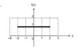
Which functional identity holds for this curve?
Show answer and explanation
Answer: (C) if f(x) = f(–x)
Reading the key coordinates on the graph:
-
At , ; at , .
-
At , ; at , .
Because is perfectly symmetric about the vertical y-axis, for all values in its domain.
Hence, is an even function, making (3) if f(x) = f(–x) the correct choice.
Question 22 · CAT Level
Directions for Questions 21 to 23
Answer the questions on the basis of the information given below.
In aerospace flight dynamics and thruster control systems, engineers evaluate piece-wise linear attitude-adjustment response functions depicted as solid lines across the normalized operational domain.
For each graph, choose the valid mathematical relation satisfied by :
-
(1) if
-
(2) if
-
(3) if
-
(4) if , for
Refer to the thruster response curve given below:
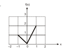
Which functional identity holds for this curve?
Show answer and explanation
Answer: (D) if 3f(x) = 6 f(–x), for x ≥ 0
Reading points for from the graph:
-
At : , while at , .
-
At : , while at , .
For all , the ratio , which translates directly to .
Hence, the correct option is (4).
Question 23 · CAT Level
Directions for Questions 21 to 23
Answer the questions on the basis of the information given below.
In aerospace flight dynamics and thruster control systems, engineers evaluate piece-wise linear attitude-adjustment response functions depicted as solid lines across the normalized operational domain.
For each graph, choose the valid mathematical relation satisfied by :
-
(1) if
-
(2) if
-
(3) if
-
(4) if , for
Refer to the thruster response curve given below:
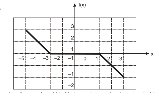
Which functional identity holds for this curve?
Show answer and explanation
Answer: (B) if f(x) = –f(–x)
Reading points across the domain:
-
At : ; at : .
-
At : ; at : .
Notice that everywhere (the graph has point symmetry through the origin , characterizing an odd function).
Hence, the correct option is (2) if f(x) = –f(–x).
Question 24 · CAT Level
Directions for Questions 24 to 29
Answer the questions on the basis of the information given below.
Precision engineering manufacturer Apex Mechatronics (ABC Ltd.) manufactures micro-actuator units (widgets) for which market demand is virtually unlimited, allowing all manufactured units to be sold immediately.
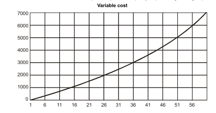
The line graph below describes the monthly variable production costs incurred by the facility as a function of the monthly output volume (units produced).
Additionally, facility operating overheads are structured into discrete production shifts:
-
Operating the production facility for the first shift results in a fixed monthly overhead cost of Rs. 800.
-
Activating a second shift incurs an additional fixed monthly overhead cost of Rs. 1,200 (bringing total fixed monthly costs to Rs. 2,000).
-
Each shift provides a maximum rated production capacity of 30 widgets per month (maximum dual-shift plant capacity is 60 widgets per month).
Key Definitions:
-
Average Unit Cost (AC) is defined as:
-
Marginal Cost (MC) represents the rate of change in total cost per additional unit produced:
If total production output in July is 40 units, what is the approximate average unit cost (AC) for the month?
Show answer and explanation
Answer: (C) 140
For a production volume of 40 units in July:
-
Shift Structure & Fixed Cost:
-
Shift 1 capacity = 30 units (Fixed Cost = Rs. 800).
-
Producing 40 units necessitates activating Shift 2 (Fixed Cost = Rs. 1,200).
-
Total Fixed Overhead .
-
-
Variable Cost:
- From the variable cost curve, at 40 units: .
-
Total Cost & Average Cost:
Hence, the approximate average unit cost is 140.
Question 25 · CAT Level
Directions for Questions 24 to 29
Answer the questions on the basis of the information given below.
Precision engineering manufacturer Apex Mechatronics (ABC Ltd.) manufactures micro-actuator units (widgets) for which market demand is virtually unlimited, allowing all manufactured units to be sold immediately.
The line graph below describes the monthly variable production costs incurred by the facility as a function of the monthly output volume (units produced).
Additionally, facility operating overheads are structured into discrete production shifts:
-
Operating the production facility for the first shift results in a fixed monthly overhead cost of Rs. 800.
-
Activating a second shift incurs an additional fixed monthly overhead cost of Rs. 1,200 (bringing total fixed monthly costs to Rs. 2,000).
-
Each shift provides a maximum rated production capacity of 30 widgets per month (maximum dual-shift plant capacity is 60 widgets per month).
Key Definitions:
-
Average Unit Cost (AC) is defined as:
-
Marginal Cost (MC) represents the rate of change in total cost per additional unit produced:
Apex Mechatronics is evaluating expanding its production throughput. What is the approximate marginal cost (MC) of increasing output from its current July operating level of 40 units?
Show answer and explanation
Answer: (B) 130
Marginal Cost (MC) is the incremental cost of producing one additional unit (from 40 to 41 units).
Because producing 41 units remains well within the second shift capacity (up to 60 units), fixed overhead costs do not change.
From the slope of the curve around 40 units:
Hence, the approximate marginal cost is 130.
Question 26 · CAT Level
Directions for Questions 24 to 29
Answer the questions on the basis of the information given below.
Precision engineering manufacturer Apex Mechatronics (ABC Ltd.) manufactures micro-actuator units (widgets) for which market demand is virtually unlimited, allowing all manufactured units to be sold immediately.
The line graph below describes the monthly variable production costs incurred by the facility as a function of the monthly output volume (units produced).
Additionally, facility operating overheads are structured into discrete production shifts:
-
Operating the production facility for the first shift results in a fixed monthly overhead cost of Rs. 800.
-
Activating a second shift incurs an additional fixed monthly overhead cost of Rs. 1,200 (bringing total fixed monthly costs to Rs. 2,000).
-
Each shift provides a maximum rated production capacity of 30 widgets per month (maximum dual-shift plant capacity is 60 widgets per month).
Key Definitions:
-
Average Unit Cost (AC) is defined as:
-
Marginal Cost (MC) represents the rate of change in total cost per additional unit produced:
Based on the cost curves provided, what can be inferred regarding the behavior of Marginal Cost (MC) for production volumes in the range of 0 to 60 units?
Show answer and explanation
Answer: (A) MC is an increasing function of production quantity.
Marginal Cost (MC) mathematically corresponds to the first derivative (slope) of the total cost / variable cost curve.
Inspecting the variable cost curve across the entire domain from 0 to 60 units, the curve is strictly convex everywhere — its tangent becomes continuously steeper as output increases.
Because the slope continually increases with higher production volumes, MC is an increasing function of production quantity.
Hence, the correct option is (1).
Question 27 · CAT Level
Directions for Questions 24 to 29
Answer the questions on the basis of the information given below.
Precision engineering manufacturer Apex Mechatronics (ABC Ltd.) manufactures micro-actuator units (widgets) for which market demand is virtually unlimited, allowing all manufactured units to be sold immediately.
The line graph below describes the monthly variable production costs incurred by the facility as a function of the monthly output volume (units produced).
Additionally, facility operating overheads are structured into discrete production shifts:
-
Operating the production facility for the first shift results in a fixed monthly overhead cost of Rs. 800.
-
Activating a second shift incurs an additional fixed monthly overhead cost of Rs. 1,200 (bringing total fixed monthly costs to Rs. 2,000).
-
Each shift provides a maximum rated production capacity of 30 widgets per month (maximum dual-shift plant capacity is 60 widgets per month).
Key Definitions:
-
Average Unit Cost (AC) is defined as:
-
Marginal Cost (MC) represents the rate of change in total cost per additional unit produced:
Suppose that each widget is sold at a fixed contract price of Rs. 150. What is the operating profit earned by Apex Mechatronics in July (producing 40 units)? (Profit is defined as sales revenue minus total production costs.)
Show answer and explanation
Answer: (C) 400
In July, output is 40 units:
-
Sales Revenue:
-
Total Production Cost:
-
Operating Profit:
Hence, the profit earned in July is 400.
Question 28 · CAT Level
Directions for Questions 24 to 29
Answer the questions on the basis of the information given below.
Precision engineering manufacturer Apex Mechatronics (ABC Ltd.) manufactures micro-actuator units (widgets) for which market demand is virtually unlimited, allowing all manufactured units to be sold immediately.
The line graph below describes the monthly variable production costs incurred by the facility as a function of the monthly output volume (units produced).
Additionally, facility operating overheads are structured into discrete production shifts:
-
Operating the production facility for the first shift results in a fixed monthly overhead cost of Rs. 800.
-
Activating a second shift incurs an additional fixed monthly overhead cost of Rs. 1,200 (bringing total fixed monthly costs to Rs. 2,000).
-
Each shift provides a maximum rated production capacity of 30 widgets per month (maximum dual-shift plant capacity is 60 widgets per month).
Key Definitions:
-
Average Unit Cost (AC) is defined as:
-
Marginal Cost (MC) represents the rate of change in total cost per additional unit produced:
Assuming the selling price remains constant at Rs. 150 per widget and profit is defined as total revenue minus total costs, at what monthly production volume does Apex Mechatronics achieve its maximum profit?
Show answer and explanation
Answer: (A) 30
We evaluate the monthly profit across the four candidate output levels:
| Output (Units) | Shifts | Sales Revenue (Rs.) | Fixed Cost (Rs.) | Variable Cost (Rs.) | Total Cost (Rs.) | Net Profit (Rs.) |
|---|---|---|---|---|---|---|
| 30 | 1 | $30 \times 150 = 4,500$ | 800 | 2,100 | 2,900 | $4500 - 2900 = \mathbf{1,600}$ |
| 40 | 2 | $40 \times 150 = 6,000$ | 2,000 | 3,600 | 5,600 | $6000 - 5600 = 400$ |
| 50 | 2 | $50 \times 150 = 7,500$ | 2,000 | 5,100 | 7,100 | $7500 - 7100 = 400$ |
| 60 | 2 | $60 \times 150 = 9,000$ | 2,000 | 7,000 | 9,000 | $9000 - 9000 = 0$ |
Operating single-shift capacity at 30 units avoids the heavy fixed overhead of shift 2 (Rs. 1,200) and escalating marginal costs, maximizing profit at Rs. 1,600 (achieved at 30 units).
Question 29 · CAT Level
Directions for Questions 24 to 29
Answer the questions on the basis of the information given below.
Precision engineering manufacturer Apex Mechatronics (ABC Ltd.) manufactures micro-actuator units (widgets) for which market demand is virtually unlimited, allowing all manufactured units to be sold immediately.
The line graph below describes the monthly variable production costs incurred by the facility as a function of the monthly output volume (units produced).
Additionally, facility operating overheads are structured into discrete production shifts:
-
Operating the production facility for the first shift results in a fixed monthly overhead cost of Rs. 800.
-
Activating a second shift incurs an additional fixed monthly overhead cost of Rs. 1,200 (bringing total fixed monthly costs to Rs. 2,000).
-
Each shift provides a maximum rated production capacity of 30 widgets per month (maximum dual-shift plant capacity is 60 widgets per month).
Key Definitions:
-
Average Unit Cost (AC) is defined as:
-
Marginal Cost (MC) represents the rate of change in total cost per additional unit produced:
For monthly production output in the range of 0 to 30 units (single-shift operation), which of the following statements is strictly correct?
Show answer and explanation
Answer: (A) AC is always higher than MC.
In the range units, only shift 1 operates (Fixed Cost = Rs. 800):
-
.
-
At : .
-
For smaller values of , the fixed overhead term is very large, keeping well above Rs. 100 throughout.
-
On the other hand, starts below Rs. 50 and reaches only about Rs. 90 at .
Because across the entire domain of 0 to 30 units, AC is always higher than MC.
Question 30 · CAT Level
Directions for Questions 30 and 31
Answer the questions on the basis of the information given below.
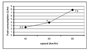
Automotive propulsion researchers evaluate fuel efficiency dynamics of the experimental prototype vehicle ‘Palto’. The fuel consumption rate (in litres per hour, L/hr) as a non-linear empirical function of cruising speed (km/hr) is characterized in the line graph below.
Test driver Manasa embarks on a 200 km highway endurance transit from Mumbai to Pune at a constant, steady cruising speed of 60 km/hr. What is the total quantity of fuel consumed during this journey?
Show answer and explanation
Answer: (B) 13.33 L
From the consumption graph:
-
At a cruising speed of , the fuel consumption rate is 4.0 L/hr.
-
Time taken to traverse 200 km at 60 km/hr:
Hence, the vehicle consumes 13.33 L.
Question 31 · CAT Level
Directions for Questions 30 and 31
Answer the questions on the basis of the information given below.
Automotive propulsion researchers evaluate fuel efficiency dynamics of the experimental prototype vehicle ‘Palto’. The fuel consumption rate (in litres per hour, L/hr) as a non-linear empirical function of cruising speed (km/hr) is characterized in the line graph below.
Manasa intends to minimize the total fuel consumed for the 200 km journey by selecting the most fuel-efficient cruising speed. How should she adjust her cruising speed relative to 60 km/hr?
Show answer and explanation
Answer: (B) Decrease the speed
We compute the total fuel required for the 200 km transit at each discrete calibrated speed marked on the curve:
| Cruising Speed | Consumption Rate | Transit Time (200 / Speed) | Total Fuel Consumed |
|---|---|---|---|
| 40 km/hr | 2.5 L/hr | 5.00 hours | $5.00 \times 2.5 = \mathbf{12.50\text{ L}}$ |
| 60 km/hr | 4.0 L/hr | 3.33 hours | $3.33 \times 4.0 = 13.33\text{ L}$ |
| 80 km/hr | 7.9 L/hr | 2.50 hours | $2.50 \times 7.9 = 19.75\text{ L}$ |
Because cruising at consumes only 12.50 L (compared to 13.33 L at 60 km/hr and 19.75 L at 80 km/hr), Manasa must decrease the speed to minimize fuel usage.
Question 32 · CAT Level
Directions for Questions 32 to 35
Answer the questions on the basis of the information given below.
In pediatric medicine and developmental biology, an infant's body length (crown-to-heel measurement in centimetres) is a primary developmental biomarker in early postnatal life. Because infants undergo continuous anatomical growth during early months, body length cannot decrease at any point in time (the growth function is monotonically non-decreasing).
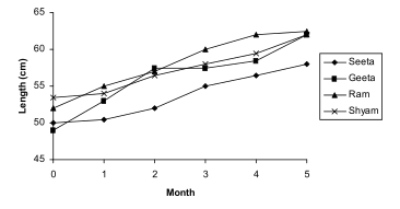
The longitudinal growth chart below traces the developmental trajectories of four infants — Geeta, Seeta, Ram, and Shyam — during their first five months of life.
After which month did Seeta's monthly rate of growth first start to decline?
Show answer and explanation
Answer: (B) Third month
The rate of anatomical growth corresponds to the slope (monthly incremental increase in length) of the curve.
Observing Seeta's growth trajectory:
-
Month 0 to 1: slope is positive.
-
Month 1 to 2: slope steepens.
-
Month 2 to 3: slope remains high.
-
Month 3 to 4: the slope noticeably flattens (decreases for the first time).
Thus, Seeta's growth rate started to decline after the third month.
Question 33 · CAT Level
Directions for Questions 32 to 35
Answer the questions on the basis of the information given below.
In pediatric medicine and developmental biology, an infant's body length (crown-to-heel measurement in centimetres) is a primary developmental biomarker in early postnatal life. Because infants undergo continuous anatomical growth during early months, body length cannot decrease at any point in time (the growth function is monotonically non-decreasing).
The longitudinal growth chart below traces the developmental trajectories of four infants — Geeta, Seeta, Ram, and Shyam — during their first five months of life.
Which of the four infants experienced the fastest rate of growth over the first two months of life (from Month 0 to Month 2)?
Show answer and explanation
Answer: (A) Geeta
The growth rate over the first two months is measured by the average slope between Month 0 and Month 2 ().
Inspecting the developmental chart, Geeta's curve displays the steepest upward slope of all four infants over , indicating the highest growth velocity during this initial phase.
Hence, Geeta grew at the fastest rate.
Question 34 · CAT Level
Directions for Questions 32 to 35
Answer the questions on the basis of the information given below.
In pediatric medicine and developmental biology, an infant's body length (crown-to-heel measurement in centimetres) is a primary developmental biomarker in early postnatal life. Because infants undergo continuous anatomical growth during early months, body length cannot decrease at any point in time (the growth function is monotonically non-decreasing).
The longitudinal growth chart below traces the developmental trajectories of four infants — Geeta, Seeta, Ram, and Shyam — during their first five months of life.
During the third month of life (between Month 2 and Month 3), the rate of growth was the lowest for which infant?
Show answer and explanation
Answer: (A) Geeta
The growth rate during the third month is given by the slope between Month 2 and Month 3.
Observing the graph over the interval, Geeta's trajectory becomes nearly flat (horizontal), indicating minimal length accumulation during this month relative to the other three infants.
Therefore, the growth rate during the third month was lowest for Geeta.
Question 35 · CAT Level
Directions for Questions 32 to 35
Answer the questions on the basis of the information given below.
In pediatric medicine and developmental biology, an infant's body length (crown-to-heel measurement in centimetres) is a primary developmental biomarker in early postnatal life. Because infants undergo continuous anatomical growth during early months, body length cannot decrease at any point in time (the growth function is monotonically non-decreasing).
The longitudinal growth chart below traces the developmental trajectories of four infants — Geeta, Seeta, Ram, and Shyam — during their first five months of life.
Among the four infants, who recorded the least relative growth over the entire five-month observation window?
Show answer and explanation
Answer: (D) Shyam
Comparing cumulative developmental growth from Month 0 to Month 5:
| Infant | Initial Length (Month 0) | Final Length (Month 5) | Absolute Growth | Percentage Growth |
|---|---|---|---|---|
| Geeta | 49 cm | 58 cm | 9 cm | $$\frac{9}{49} \approx 18.37\%$$ |
| Ram | 52 cm | 60 cm | 8 cm | $$\frac{8}{52} \approx 15.38\%$$ |
| Seeta | 50 cm | 57 cm | 7 cm | $$\frac{7}{50} = 14.00\%$$ |
| Shyam | 53 cm | 60 cm | 7 cm | $$\frac{7}{53} \approx \mathbf{13.21\%}$$ |
Both Seeta and Shyam gained 7 cm in absolute length, but Shyam started from a longer baseline (53 cm vs 50 cm), resulting in the lowest relative growth percentage (13.21%). Hence, Shyam grew the least.
Question 36 · CAT Level
Directions for Questions 36 to 38
Answer the questions on the basis of the information given below.
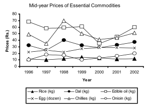
An agricultural economics monitoring agency tracks annual mid-year benchmark spot prices (in Rs. per unit) of six core essential consumer commodities — Chillies, Onion, Egg, Dal, Rice, and Edible oil — across seven consecutive years from 1996 to 2002 as displayed in the multi-line chart below.
During the period 1996–2002, the number of commodities that exhibited a net overall price increase and a net overall price decrease from their initial 1996 levels, respectively, were:
Show answer and explanation
Answer: (C) 4 and 2
Comparing the initial benchmark price in 1996 with the final terminal price in 2002 for all six commodities:
| Commodity | Price in 1996 | Price in 2002 | Net Direction |
|---|---|---|---|
| Chillies | ~10 | ~22 | Net Increase |
| Onion | ~10 | ~17 | Net Increase |
| Egg | ~12 | ~18 | Net Increase |
| Dal | ~32 | ~42 | Net Increase |
| Rice | ~14 | ~13 | Net Decrease |
| Edible oil | ~42 | ~38 | Net Decrease |
Thus, exactly 4 commodities recorded a net price increase, and 2 commodities recorded a net price decrease.
Question 37 · CAT Level
Directions for Questions 36 to 38
Answer the questions on the basis of the information given below.
An agricultural economics monitoring agency tracks annual mid-year benchmark spot prices (in Rs. per unit) of six core essential consumer commodities — Chillies, Onion, Egg, Dal, Rice, and Edible oil — across seven consecutive years from 1996 to 2002 as displayed in the multi-line chart below.
How many commodities experienced a continuous price decline across two or more consecutive yearly intervals during the period 1996–2002?
Show answer and explanation
Answer: (D) 5
We check each commodity for at least two consecutive yearly decreases ():
-
Chillies: Declines from 1998 to 1999, and 1999 to 2000 (2 consecutive years). (Yes)
-
Onion: Declines from 1998 to 1999, and 1999 to 2000 (2 consecutive years). (Yes)
-
Egg: Declines from 1997 to 1998, and 1998 to 1999 (2 consecutive years). (Yes)
-
Dal: Declines from 1999 to 2000, and 2000 to 2001 (2 consecutive years). (Yes)
-
Rice: Declines across several consecutive years. (Yes)
-
Edible oil: Experiences only single-year dips followed by recoveries/stabilization. (No)
Except Edible oil, all other 5 commodities exhibited a price decline lasting two or more consecutive years.
Question 38 · CAT Level
Directions for Questions 36 to 38
Answer the questions on the basis of the information given below.
An agricultural economics monitoring agency tracks annual mid-year benchmark spot prices (in Rs. per unit) of six core essential consumer commodities — Chillies, Onion, Egg, Dal, Rice, and Edible oil — across seven consecutive years from 1996 to 2002 as displayed in the multi-line chart below.
For which commodity/commodities did an immediate price increase follow a price decline exactly once across the entire 1996–2002 timeline?
Show answer and explanation
Answer: (D) Egg and onion
We search for a 'trough' or valley pattern (where a downward line segment is immediately followed by an upward line segment) that occurs exactly once between 1996 and 2002:
-
Egg: Declines through 1999, then increases in 2000 — this recovery trough happens only once. (Satisfies condition)
-
Onion: Declines through 2000, then rises in 2001 — this recovery trough happens only once. (Satisfies condition)
The other commodities either experience multiple rebound troughs or different cycling behaviors.
Hence, the condition is satisfied by Egg and onion.
Question 39 · CAT Level
Directions for Questions 39 to 42
Answer the questions on the basis of the information given below.
A socio-economic household survey evaluates monthly income and expenditure patterns of individual working members across four extended urban family cohorts: Ahuja, Bose, Coomar, and Dubey.
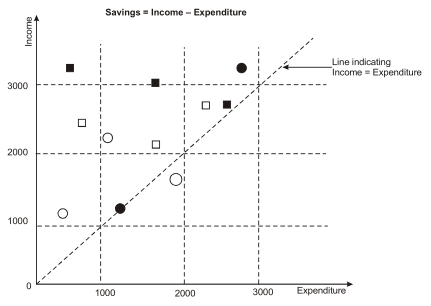
In the scatter/coordinate graph below, each point represents the financial coordinates of a single individual member, labeled by family surname and numeric index (e.g., Ahuja1, Ahuja2, Ahuja3, etc.). Both income (vertical axis) and expenditure (horizontal axis) are measured in rupees.
In all questions, monthly savings is defined as:
Which family cohort has the lowest average monthly income across its individual members?
Show answer and explanation
Answer: (C) Coomar
Reading monthly income (y-axis coordinate) for all members of each family cohort:
| Family Cohort | Working Members | Individual Incomes (Rs.) | Total Family Income (Rs.) | Average Monthly Income (Rs.) |
|---|---|---|---|---|
| Ahuja | 3 | 3,200; 3,000; 2,800 | 9,000 | $$\frac{9000}{3} = 3,000$$ |
| Bose | 3 | 2,300; 2,100; 2,800 | 7,200 | $$\frac{7200}{3} = 2,400$$ |
| Coomar | 3 | 1,200; 2,200; 1,600 | 5,000 | $$\frac{5000}{3} \approx \mathbf{1,667}$$ |
| Dubey | 2 | 1,200; 3,200 | 4,400 | $$\frac{4400}{2} = 2,200$$ |
The Coomar family has the lowest average income (~Rs. 1,667).
Question 40 · CAT Level
Directions for Questions 39 to 42
Answer the questions on the basis of the information given below.
A socio-economic household survey evaluates monthly income and expenditure patterns of individual working members across four extended urban family cohorts: Ahuja, Bose, Coomar, and Dubey.
In the scatter/coordinate graph below, each point represents the financial coordinates of a single individual member, labeled by family surname and numeric index (e.g., Ahuja1, Ahuja2, Ahuja3, etc.). Both income (vertical axis) and expenditure (horizontal axis) are measured in rupees.
In all questions, monthly savings is defined as:
Which family cohort has the highest average monthly expenditure across its individual members?
Show answer and explanation
Answer: (D) Dubey
Reading monthly expenditure (x-axis coordinate) for all members of each family cohort:
| Family Cohort | Working Members | Individual Expenditures (Rs.) | Total Expenditure (Rs.) | Average Expenditure (Rs.) |
|---|---|---|---|---|
| Ahuja | 3 | 700; 1,700; 2,700 | 5,100 | $$\frac{5100}{3} = 1,700$$ |
| Bose | 3 | 800; 1,750; 2,300 | 4,850 | $$\frac{4850}{3} \approx 1,617$$ |
| Coomar | 3 | 500; 1,100; 1,900 | 3,500 | $$\frac{3500}{3} \approx 1,167$$ |
| Dubey | 2 | 1,200; 2,800 | 4,000 | $$\frac{4000}{2} = \mathbf{2,000}$$ |
The Dubey family records the highest average monthly expenditure (Rs. 2,000).
Question 41 · CAT Level
Directions for Questions 39 to 42
Answer the questions on the basis of the information given below.
A socio-economic household survey evaluates monthly income and expenditure patterns of individual working members across four extended urban family cohorts: Ahuja, Bose, Coomar, and Dubey.
In the scatter/coordinate graph below, each point represents the financial coordinates of a single individual member, labeled by family surname and numeric index (e.g., Ahuja1, Ahuja2, Ahuja3, etc.). Both income (vertical axis) and expenditure (horizontal axis) are measured in rupees.
In all questions, monthly savings is defined as:
Which family cohort records the lowest average monthly savings across its individual members?
Show answer and explanation
Answer: (D) Dubey
Average savings is computed as :
| Family Cohort | Average Income (Rs.) | Average Expenditure (Rs.) | Average Monthly Savings (Rs.) |
|---|---|---|---|
| Ahuja | 3,000 | 1,700 | $3000 - 1700 = 1,300$ |
| Bose | 2,400 | 1,617 | $2400 - 1617 = 783$ |
| Coomar | 1,667 | 1,167 | $1667 - 1167 = 500$ |
| Dubey | 2,200 | 2,000 | $2200 - 2000 = \mathbf{200}$ |
The Dubey family has the lowest average monthly savings (Rs. 200).
Question 42 · CAT Level
Directions for Questions 39 to 42
Answer the questions on the basis of the information given below.
A socio-economic household survey evaluates monthly income and expenditure patterns of individual working members across four extended urban family cohorts: Ahuja, Bose, Coomar, and Dubey.
In the scatter/coordinate graph below, each point represents the financial coordinates of a single individual member, labeled by family surname and numeric index (e.g., Ahuja1, Ahuja2, Ahuja3, etc.). Both income (vertical axis) and expenditure (horizontal axis) are measured in rupees.
In all questions, monthly savings is defined as:
The highest absolute monthly savings accrues to an individual member belonging to which family?
Show answer and explanation
Answer: (A) Ahuja
An individual's savings equals the vertical distance of their coordinate point above the 45-degree diagonal line representing ():
-
The point with the largest vertical clearance above this line is a member of the Ahuja family (Ahuja1):
No other individual across any family approaches a monthly savings margin of Rs. 2,500.
Hence, the highest savings accrues to a member of the Ahuja family.
Question 43 · CAT Level
Directions for Questions 43 to 45
Answer the questions on the basis of the information given below.
Telecommunications network operators generate top-line gross revenue through the transmission of voice calls and packetized data services. The average unit realization received per unit volume of data transferred is termed ARDT (Average Revenue per Data Unit Transferred, in USD).
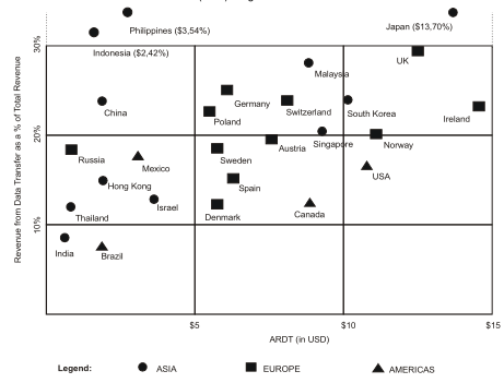
In the bubble chart below, each plotted entity represents an individual nation in the year 2007:
-
The coordinates and bracketed values indicate the ARDT and the revenue from data transfer expressed as a percentage of the country's total telecommunications revenue.
-
The area / size of each bubble is proportional to the total telecommunications revenue generated in that country in 2007.
Suppose it was determined that the total physical volume of data transferred in India was equal to that of Singapore in 2007. Which of the following statements correctly characterizes their total telecommunications revenues?
Show answer and explanation
Answer: (D) Total revenue in Singapore is about 4 time that of India.
Let the equal physical volume of data transferred in India and Singapore be .
-
For India:
-
-
Data Revenue
-
Data Revenue is approximately of Total Revenue
-
-
For Singapore:
-
-
Data Revenue
-
Data Revenue is approximately of Total Revenue
-
-
Comparison:
Therefore, the Total Revenue in Singapore is about 4 times that of India.
Question 44 · CAT Level
Directions for Questions 43 to 45
Answer the questions on the basis of the information given below.
Telecommunications network operators generate top-line gross revenue through the transmission of voice calls and packetized data services. The average unit realization received per unit volume of data transferred is termed ARDT (Average Revenue per Data Unit Transferred, in USD).
In the bubble chart below, each plotted entity represents an individual nation in the year 2007:
-
The coordinates and bracketed values indicate the ARDT and the revenue from data transfer expressed as a percentage of the country's total telecommunications revenue.
-
The area / size of each bubble is proportional to the total telecommunications revenue generated in that country in 2007.
Industry projections forecast that by 2010, revenue from data transfer as a percentage of total revenue will triple for India and double for Sweden. Assuming that in 2010, the total revenue in India is twice that of Sweden and the physical volume of data transfer is identical in both nations, what will be the percentage increase in India's ARDT if Sweden's ARDT remains constant at its 2007 level?
Show answer and explanation
Answer: (C) 800%
Let Sweden's total revenue in 2010 be .
Then India's total revenue in 2010 is .
-
Sweden in 2010:
-
Data revenue percentage doubles from to .
-
-
ARDT remains constant at .
-
-
India in 2010:
-
Data revenue percentage triples from to .
-
-
Given that data volume is identical: .
-
-
Percentage Increase in India's ARDT:
Hence, India's ARDT increases by 800%.
Question 45 · CAT Level
Directions for Questions 43 to 45
Answer the questions on the basis of the information given below.
Telecommunications network operators generate top-line gross revenue through the transmission of voice calls and packetized data services. The average unit realization received per unit volume of data transferred is termed ARDT (Average Revenue per Data Unit Transferred, in USD).
In the bubble chart below, each plotted entity represents an individual nation in the year 2007:
-
The coordinates and bracketed values indicate the ARDT and the revenue from data transfer expressed as a percentage of the country's total telecommunications revenue.
-
The area / size of each bubble is proportional to the total telecommunications revenue generated in that country in 2007.
Assuming that total gross revenue received is identical for the paired countries listed below, which pair has approximately the same physical volume of data transfer?
Show answer and explanation
Answer: (D) UK and Spain
Physical volume of data transfer is given by:
If Total Revenue is identical for both countries in a pair, volume is directly proportional to .
Evaluating the ratio across the candidate pairs:
| Country | Data Revenue % | ARDT (USD) | Volume Ratio (Data% / ARDT) |
|---|---|---|---|
| UK | ~30% | $13 | $$\frac{30}{13} \approx \mathbf{2.31}$$ |
| Spain | ~15% | $6.5 | $$\frac{15}{6.5} \approx \mathbf{2.31}$$ |
| Philippines | ~54% | $3.0 | $$\frac{54}{3} = 18.0$$ |
| Austria | ~19% | $6.0 | $$\frac{19}{6} \approx 3.17$$ |
| Canada | ~14% | $8.0 | $$\frac{14}{8} = 1.75$$ |
| Poland | ~21% | $5.5 | $$\frac{21}{5.5} \approx 3.82$$ |
| Germany | ~22% | $6.0 | $$\frac{22}{6} \approx 3.67$$ |
| USA | ~16% | $10.0 | $$\frac{16}{10} = 1.60$$ |
UK and Spain yield an identical volume ratio of 2.31, meaning they have approximately the same physical volume of data transfer.
Try real CAT questions
Study this concept with interactive practice in PrepSoc.
Open the concept library